>

WAVEFORMS TUTORIAL

Gravitational Waves

SimulationTools has a large set of functionality for working with numerical time-series waveforms such as one would obtain by extracting gravitational radiation from a numerical relativity simulation.

Reading and exporting waveforms

SimulationTools supports a plug-in interface for reading waveform data. The format of choice is HDF5 data using the naming conventions of the Multipole Cactus thorn which is included with the Einstein Toolkit. There is also support for reading waveforms as ASCII data produced by the Multipole thorn and for reading waveforms in the NRDF format [http://arxiv.org/abs/0709.0093].

Reading data in Multipole format

Reading data produced using the Multipole Cactus thorn.

Read in the (2,2) mode of the gravitational waveform from a binary black hole merger, represented by extracted at a radius of 100M

In[1]:=

In[4]:=

Out[4]=

It is possible to specify the name of the output file produced by the Multipole thorn using the Multipole::variables parameter in the simulation parameter file, e.g.

    Multipole::variables = “WeylScal4::Psi4r{sw=-2 cmplx=’WeylScal4::Psi4i’ name=’psi4’}”

By default, it is assumed that the name ‘psi4’ is used. This may be changed by setting $MultipolePsi4Variable

In[5]:=

In[6]:=

Out[6]=

Waveforms can be produced for multiple (l,m) modes and multiple extraction radii. The list of available modes and radii are both easily accessed

In[7]:=

Out[7]=

In[8]:=

Out[8]=

Reading waveforms in other formats

Waveform data from other sources can be imported in a standard ASCII format with three columns corresponding to time and the real and imaginary parts of the waveform

In[9]:=

In[10]:=

Out[10]=

Exporting waveforms

Waveforms can be easily exported as ASCII files

In[11]:=

Out[11]=

Working with waveforms

Visualisation

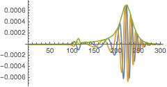
Plot the real and imaginary parts along with the absolute value

In[12]:=

Out[12]=

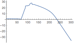
Plot the phase of the complex waveform

In[13]:=

Out[13]=

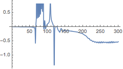
and plot the frequency

In[14]:=

Out[14]=

One frequently would like to know how many gravitational wave cycles are present in a waveform as a measure of its length. The WaveformCycles function does so by counting the number of oscillations from a prescribed time up to the peak of the amplitude, which is assumed to correspond to the merger. In the short example binary black hole simulation, there are approximately three gravitational wave cycles before the merger.

In[15]:=

Out[15]=

It is also possible to obtain this number directly from the simulation, without having to go through the step of reading explicitly

In[16]:=

Out[16]=

Manipulating waveforms

Aligning phases

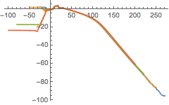
It is often convenient to consider a complex waveform in terms of amplitude and phase rather than real and imaginary parts.  When computing the phase, there is a freedom to add multiples of 2π.  When compare two different waveforms, it’s possible that different multiples of 2π have been added to each (this usually happens when the data is not smooth and the algorithm to produce a continuous phase in the Phase function makes a different choice for different waveforms).  The AlignedPhases function adds multiples of 2π to a set of phases to minimise their difference at a specific time.

In[17]:=

In[21]:=

Out[21]=

Converting to strain

Waveforms from numerical relativity simulations are typically extracted as the complex scalar , whereas many analytic and data analysis calculations prefer to work with the strain, h, which is related to by two time integrals. The function Psi4ToStrain does this conversion using either fixed-frequency or time-domain integration methods.

Convert to h using fixed-frequency integration

In[22]:=

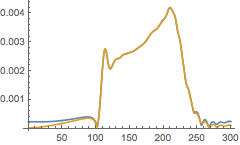
Convert to h using time domain integration chosing the two arbitrary integration constants such that the strain is 0 at t=0 and t=280

In[24]:=

Compare the two integration schemes

In[25]:=

Out[25]=

Extrapolation

Waveforms from numerical simulations are normally obtained by extraction of at finite radius. However, their definition is in terms of at future null infinity.  It is therefore common to extract at a sequence of radii and extrapolate to infinite radius. SimulationTools provides some automated functions for performing such an extrapolation.

The function ReadRadiallyExtrapolatedPsi4 reads a specific (l,m) mode of at all radii available in a simulation and produces a waveform which has been extrapolated to infinite radius

In[26]:=

In[27]:=

Out[27]=

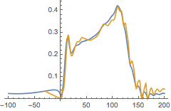
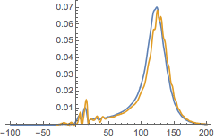
We can compare this extrapolated waveform to the one extracted at r=100M

In[28]:=

Out[28]=

One may also wish to compute the strain at future null infinity. This involves a delicate combination of conversion from to strain and extrapolation. The function ReadRadiallyExtrapolatedStrain does this in a way that has been found to be generally robust

In[29]:=

In[30]:=

Out[30]=

Related Tutorials

SimulationTools

Binaries

BlackHoles