![]() >
> ![]()
| SIMULATIONTOOLS TUTORIAL |
Convergence Testing
Many simulations involve the solution of partial differential equations using finite difference methods on a coordinate grid. Several simulations, identical apart from the grid spacing, are then compared to see how the numerical solution changes with the grid spacing. This is done both to show that the solution converges to an exact solution, and to assess the numerical error.
SimulationTools contains several functions to help in this process.
In the examples below, we will use a set of three DataTables constructed to simulate a second-order accurate numerical solution to some partial differential equation.
The grid spacings are
In[1]:=
![]()
The “numerical solutions” are
In[2]:=
![]()
Out[2]=
![]()
In[3]:=
![]()
Out[3]=
![]()
In[4]:=
![]()
Out[4]=
![]()
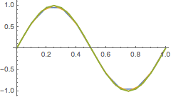
We can plot the DataTables directly:
In[5]:=
![]()
Out[5]=

Ratio between solution differences
Assuming convergence of the numerical solutions at a given order, the ratio between the differences of numerical solutions, ![]() and
and ![]() is given by
is given by
![]()
This is accurate to order p+1.
In[6]:=
![]()
Out[6]=
![]()
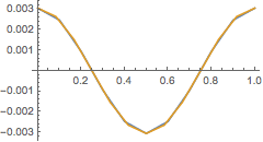
For the example above, we can confirm that the data satisfies this property by plotting the two differences, with the second one rescaled by the convergence multiplier:
In[7]:=
![]()
Out[7]=
![]()
In[8]:=
![]()
Out[8]=

The two curves lie on top of each other, since the convergence is exactly 2nd order in this case.
The WithResampling function is necessary in order for subtraction of DataTables on different coordinate grids to use interpolation automatically (the interpolation is 8th order by default).
Convergence rate
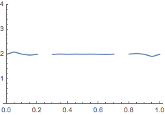
You can also measure the convergence rate:
In[9]:=
![]()
Out[9]=

Note that the convergence rate cannot be determined at the points where ![]()
For general ![]() ,
, ![]() and
and ![]() , the convergence rate cannot be solved for exactly; Mathematica’ FindRoot function is used to solve the algebraic equation. As such, in certain cases a solution might not be found.
, the convergence rate cannot be solved for exactly; Mathematica’ FindRoot function is used to solve the algebraic equation. As such, in certain cases a solution might not be found.
RichardsonExtrapolant
Assuming a given order of convergence, you can use two of the solutions to estimate a higher-order approximation of the exact solution. This is called Richardson Extrapolation and is useful for providing an error estimate in one of the numerical solutions. The RichardsonExtrapolant function gives this estimate:
In[10]:=
![]()
Out[10]=
![]()
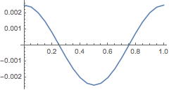
An error estimate (accurate to 3rd order) for f3 can be determined by subtracting the Richardson extrapolant:
In[11]:=
![]()
Out[11]=
![]()
In[12]:=
![]()
Out[12]=
