>

SIMULATIONTOOLS TUTORIAL

Advanced Analysis

Once simulation data has been loaded into Mathematica as DataTable or DataRegion objects, the full power of Mathematica can be used.  The data can remain in discrete form, for example as a DataRegion, or it can be interpolated to provide a continuous function.  In the latter case, it can be used with functions like NDSolve, NIntegrate, FindRoot etc.  We now give some examples of more sophisticated data analysis that can be performed with simulation data.

Line Integral

The first example is to integrate the grid function phi along the line joining the two black holes in the example data.  (This has no physical significance; it’s just a demonstration.)

Load the data:

In[1]:=

Out[1]=

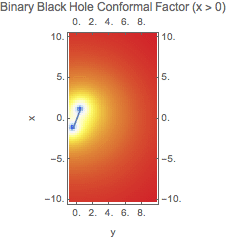
Plot the data:

In[2]:=

Out[2]=

Construct a 2-dimensional interpolating function from the data:

In[3]:=

Out[3]=

The coordinate time of this data:

In[4]:=

Out[4]=

The coordinate positions of the black holes at this time:

In[5]:=

Out[5]=

In[6]:=

Out[6]=

The line joining the two can be expressed in parametric form

In[7]:=

Out[7]=

and used in ParametricPlot.  Mathematica plots can be combined using Show:

In[8]:=

Out[8]=

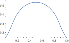
We can now plot phi along this line:

In[9]:=

Out[9]=

Note that the @@ (Apply) is needed because the InterpolatingFunction phiFn takes two separate coordinate arguments, whereas bhLine is a list containing the two coordinates.

Finally, we can compute the integral along the line:

In[10]:=

Out[10]=

In[11]:=

Out[11]=

Surface Integral

We can compute surface integrals in a similar way.  First load a 3D data set:

In[12]:=

Out[12]=

In[13]:=

Out[13]=

Find the initial position of the first black hole:

In[14]:=

Out[14]=

Interpolate the 3D data:

In[15]:=

Out[15]=

Choose a surface of radius 2 centred on the black hole:

In[16]:=

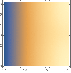
Plot phi as a function of θ and φ:

In[17]:=

Out[17]=

Compute the surface integral:

In[18]:=

Out[18]=

(The warnings are a result of the poor convergence of the numerical integral on discretely-sampled data)